- 统一精排阶段的特征交叉和序列建模
- 多目标优化对齐
- 利用PRM监督生成式推荐模型
- 个性化搜索中的知识-动作对齐
- 生成式推荐系统中的预测解码加速

一、Motivation
LLM 中拥有丰富的语义知识,理论上非常适合为个性化搜索系统注入语义泛化能力。但淘宝团队在实践中发现,直接对 LLM 进行个性化任务微调,效果往往不尽如人意。
研究团队发现核心问题在于Knowledge-Action Gap,即 LLM 预训练获得的丰富语义知识与个性化任务中的判别性目标(如点击预测)存在内在冲突:过度优化 Action 会严重扭曲预训练的语义空间,而冻结 LLM 又会导致表征过于粗糙,无法有效个性化。
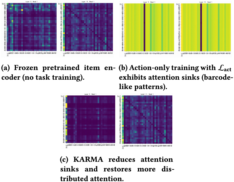
更严重的是,如果将每个物品压缩为单个 embedding,会出现 Semantic Collapse。此时注意力图退化成条形码状的模式,造成 attention sink 现象,模型就会用 ID 式特征而非真正的语义建模。
二、KARMA
KARMA (Knowledge-Action Regularized Multimodal Alignment) 的核心思想:将语义重建作为训练时的正则化器。
- 为了更好地排序,表征应该与用户的动作对齐
- 为了保持语义知识,表征也应该具有可解码性,能够还原出目标物品的原始语义
为此,KARMA设计了以下目标函数:
\[\begin{equation} \mathcal{L}=\mathcal{L}_{\mathrm{act}}+\lambda_{\mathrm{dec}}\mathcal{L}_{\mathrm{dec}} \end{equation}\]其中,$\mathcal{L}{\mathrm{act}}$ 是动作对齐目标,用于提高召回和排序的精度,$\mathcal{L}{\mathrm{dec}}$ 是可解码性正则化项,用于保持语义知识。
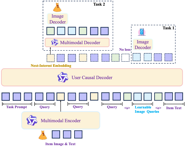
KARMA 的关键设计思想是 Train-Heavy, Infer-Light,所有解码头仅在训练时使用,不会增加任何推理延迟。
2.1. 动作对齐目标
给定 query 表征 $\mathbf{h}t$,正样本为 ground-truth 物品 $i_t$ 的表征 $\mathbf{e}{i_t}$,负样本 $\lbrace\mathbf{e}j\rbrace{j\in\mathcal{N}_t}$ 有两种:难负样本(曝光未点击)和 in-batch 负样本。动作对齐目标使用成对交叉熵损失:
\[\begin{equation} \mathcal{L}_{\mathrm{act}}= \sum_t\sum_{j\in\mathcal{N}_t}-\log\sigma\left( \mathbf{h}_t^\top\mathbf{e}_{i_t} -\mathbf{h}_t^\top\mathbf{e}_j \right) \end{equation}\]这种方式会比 InfoNCE 更加稳定。
2.2. 可解码性正则化项
$\mathcal{L}_{\mathrm{dec}}$ 中包括了两个互补的可解码性目标。
2.2.1. History-conditioned Semantic Generation
令 ground-truth 物品的描述文本为 $y_{i_t}=\lbrace w_1, \cdots, w_L\rbrace$。这个目标从行为历史 $\mathcal{H}_t$ 直接解码描述文本:
\[\begin{equation} \mathcal{L}_{\mathrm{gen}}=-\log p_\theta(w_l \mid w_{\lt l}, \mathcal{H}_t) \end{equation}\]这种方式将训练锚定到 LLM 原生的 token 分布,缓解了灾难性遗忘。
2.2.2. Embedding-conditioned Semantic Reconstruction
这个目标要求 next-interest embedding 也是语义可解码的:
\[\begin{equation} \mathcal{L}_{\mathrm{recon}}=-\log p_\theta(w_l \mid w_{\lt l}, \mathbf{h}_t) \end{equation}\]通过强制 embedding bottleneck,防止模型走 ID 式捷径。
2.2.3. 多模态扩展
当有多模态监督时,还可以使用条件 diffusion 或 flow matching 模型来重建视觉特征 $\mathbf{v}_{i_t}$。
\[\begin{equation} \mathcal{L}_{\mathrm{img}}=\mathbb{E}_{\tau}\lbrack \ell_{\mathrm{diff}}\left( g_{\psi};\mathbf{v}_{i_t},\mathbf{c}_t,\tau \right) \rbrack \end{equation}\]其中,$\mathbf{c}_t$ 表示条件信号,即行为历史 $\mathcal{H}_t$ 或者 next-interest embedding $\mathbf{h}_t$。
Experiment
3.1. 离线实验
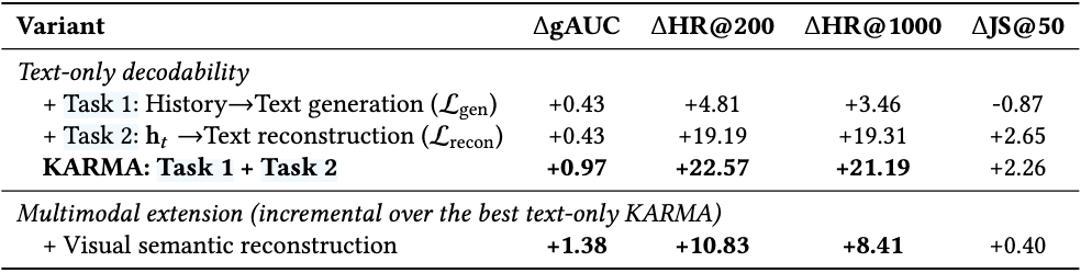
关键发现:
- Action-only 训练容易走捷径,语义保真度很低(JS@50)
- 两个正则化项互补,联合使用效果最佳。Embedding-conditioned 可解码性是主要的反坍塌约束
3.2. Mode-Mean Dilemma
有趣的是,论文发现扩散模型不适合作为检索 embedding 的生成器:
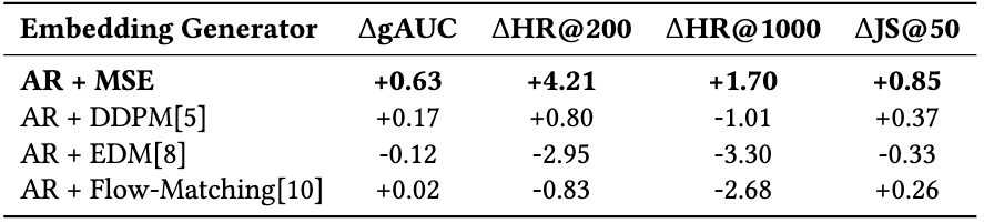
作者分析认为,扩散目标是 mode-seeking(采样高保真实例),而检索 embedding 需要 mean-seeking(作为稳定中心聚合多个可能的未来意图),这两者存在根本冲突。但作为语义正则化器,扩散模型的 mode-seeking 性质反而提供了有益的归纳偏置,帮助防止语义坍塌。
在附录中,我们从多个角度证明了这个结论。
3.3. 线上实验
KARMA 在淘宝搜索系统的三个阶段部署:
- 召回:+2.51 HR@5000
- 粗排:+1.86 HR@500
- 精排:+0.25 CTR AUC
14 天 A/B 测试:GMV +0.9%,且推理开销为零。
Appendix
为什么扩散模型适合做语义正则化器?
作为正则化器时,扩散模型的 mode-seeking 性质反而成为优势。我们从以下几个方面进行证明。
1. 流形正则化效应
假设商品图像、文本等自然数据分布在 $\mathbb{R}^D$ 的某个低维流形 $\mathcal{M} \subset \mathbb{R}^D$ 上。扩散模型的重建损失隐式地施加了流形正则化,要求模型学到的表示必须与数据流形的得分函数一致。
\[\begin{equation} \mathcal{L}_{\mathrm{diff}} = \mathbb{E}_{t, x_0, \epsilon} \left[ \Vert \nabla_{x_t} \log p_t(x_t) - \epsilon_\theta(x_t, t) \Vert ^2 \right] \end{equation}\]其中 $p_t$ 是数据在时间 $t$ 的扰动分布。
当用作正则化器时,我们优化: \(\min_\theta \mathcal{L}_{\mathrm{task}} + \lambda \mathcal{L}_{\mathrm{diff}}(\theta)\)
这等价于在参数空间施加约束: \(\begin{equation} \theta \in \{ \theta : \mathbb{E}_{x \sim \mathcal{M}}[\Vert \nabla_x \log p(x) - \nabla_x \log p_\theta(x) \Vert ^2] \leq \epsilon \} \end{equation}\)
这防止了表示偏离数据流形,避免学习到奇异的、不在流形上的表征。
2. 隐式谱偏差(Spectral Bias)
扩散模型作为正则化器时,具有低频优先的谱偏差,这有利于语义稳定性。
考虑扩散过程的频域分析。设数据的傅里叶分解为
\[\begin{equation} x = \sum_{k=0}^{\infty} \hat{x}_k \phi_k \end{equation}\]扩散前向过程在时域上表示为:
\[\begin{equation} x_t = \sqrt{\bar{\alpha}_t} x_0 + \sqrt{1-\bar{\alpha}_t} \epsilon \end{equation}\]在频域上则表示为:
\[\begin{equation} \hat{x}_t(k) = \sqrt{\bar{\alpha}_t} \hat{x}_0(k) + \sqrt{1-\bar{\alpha}_t} \hat{\epsilon}(k) \end{equation}\]这里能得到一个关键结论:高频分量衰减更快。因为高频对应细节,低频对应语义结构。
在反向去噪过程中,优先恢复的是低频分量:
\[\begin{equation} \mathbb{E}[\hat{x}_{\mathrm{recon}}(k)] \approx \begin{cases} \hat{x}_0(k) & k \mathrm{ is low frequency} \\ 0 & k \mathrm{ is high frequency} \end{cases} \end{equation}\]作为正则化器,这相当于只约束低频(语义)分量,忽略高频(噪声)分量:
\[\begin{equation} \mathcal{L}_{\mathrm{diff}} \approx \sum_{k \in \mathrm{low}} \lVert \hat{h}(k) - \hat{v}(k) \rVert^2 + \mathrm{const} \end{equation}\]这解释了为什么扩散模型能有效防止语义坍塌:它天然关注语义结构,而非表面细节。
3. 互信息最大化
扩散模型正则化近似最大化表征向量与语义的互信息。
考虑 InfoNCE 下界:
\[\begin{equation} I(h; v) \geq \mathbb{E}[\log p(\mathbf{v}\mid \mathbf{h})] + H(\mathbf{v}) \end{equation}\]扩散模型的重建损失为:
\[\begin{equation} \mathcal{L}_{\mathrm{recon}} = -\mathbb{E}[\log p_\theta(\mathbf{v}\mid \mathbf{h})] \end{equation}\]最小化 $\mathcal{L}{\mathrm{recon}}$ 等价于最大化 $\mathbb{E}[\log p\theta(\mathbf{v}\mid \mathbf{h})]$,即最大化互信息的下界。这意味着,扩散正则化强制表征 $\mathbf{h}$ 与语义 $\mathbf{v}$ 的互信息最大。
action-only 的训练方式只最大化 $\mathbf{h}$ 与标签 $\mathbf{y}$ 的互信息,可能丢弃与 $\mathbf{y}$ 无关但与语义 $\mathbf{v}$ 相关的信息。 \(\begin{equation} \mathcal{L}_{\mathrm{act}} = -\mathbb{E}[\log p(\mathbf{y}\mid \mathbf{h})] \end{equation}\)
KARMA 同时最大化 $I(\mathbf{h}; \mathbf{y})$ 和 $I(\mathbf{h}; \mathbf{v})$,学到既判别又语义丰富的表示。
4. 防止表征坍塌
给定表征 $\mathbf{h}\in \mathbb{R}^D$,其有效维度定义为协方差矩阵特征值分布的参与数 (participant number):
\[\begin{equation} \begin{aligned} P &:=\frac{\mathrm{Tr}(\mathrm{Cov}(\mathbf{h}))^2}{\mathrm{Tr}(\mathrm{Cov}(\mathbf{h})^2)}\\ &=\frac{\left(\sum_{i}\lambda_i\right)^2}{\sum_{i}\lambda_i^2} \end{aligned} \end{equation}\]其中,$\lambda_i$ 是 $\mathrm{Cov}(\mathbf{h})$ 的特征值。
- 当所有特征值都相同时,$P=D$,此时数据在各个方向上方差相同,占据整个空间。
- 当只有 $k$ 个非零特征值时,$P=k$,此时数据坍缩到一个 $k$ 维流形上。
表征坍缩 (Representation Collapse) 是指表征的有效维度 $P\ll D$,此时表征的协方差矩阵仅有几个非0特征值,坍缩到一个低维流形上。
当扩散模型的重建损失很小时,表征的协方差矩阵的最小特征值存在下界。这使得协方差矩阵不会退化为奇异矩阵,有效维度不会太小,从而防止了表征坍塌。
设扩散重建损失为: \(\begin{equation} \mathcal{L}_{\mathrm{diff}} = \mathbb{E}[\Vert \mathbf{v} - D(\mathbf{h}) \Vert ^2] \end{equation}\)
其中 $\mathbf{v} \in \mathbb{R}^{d_v}$ 是目标语义,$\mathbf{h} \in \mathbb{R}^{d_h}$ 是表征,$D(h) = Wh + b$ 是线性解码器。
1. 求解最优线性解码器
首先对 $b$ 求导: \(\begin{equation} \frac{\partial \mathcal{L}}{\partial b} = -2(\mathbb{E}[\mathbf{v}] - W\mathbb{E}[\mathbf{h}] - b) \end{equation}\)
令导数为0,解得最优偏置为:
\[\begin{equation} b^{\ast} = \mathbb{E}[\mathbf{v}] - W\mathbb{E}[\mathbf{h}] \end{equation}\]将重构损失展开并使用迹的性质:
\[\begin{equation} \mathcal{L}_{\mathrm{diff}} = \mathrm{Tr}(\mathrm{Cov}(\mathbf{v})) - 2\mathrm{Tr}(W \mathrm{Cov}(\mathbf{h}, \mathbf{v})) + \mathrm{Tr}(W^\top W \mathrm{Cov}(\mathbf{h})) \end{equation}\]对 $W$ 求导得:
\[\begin{equation} \frac{\partial \mathcal{L}}{\partial W} = -2\mathrm{Cov}(\mathbf{h}, \mathbf{v})^\top + 2\mathrm{Cov}(\mathbf{h})W^\top \end{equation}\]假设 $\mathrm{Cov}(\mathbf{h})$ 可逆,令导数为0,解得最优权重:
\[\begin{equation} W^{\ast} = \mathrm{Cov}(\mathbf{v}, \mathbf{h}) \mathrm{Cov}(\mathbf{h})^{-1} \end{equation}\]2. 最小重建损失
将 $W^{\ast}$ 代入损失函数:
\[\begin{equation} \begin{aligned} \mathcal{L}_{\mathrm{diff}}^{\ast} &= \mathrm{Tr}(\mathrm{Cov}(\mathbf{v})) - 2\mathrm{Tr}(W^{\ast} \mathrm{Cov}(\mathbf{h}, \mathbf{v})) + \mathrm{Tr}(W^{*\top} W^{\ast} \mathrm{Cov}(\mathbf{h})) \\ &= \mathrm{Tr}(\mathrm{Cov}(\mathbf{v})) - 2\mathrm{Tr}(\mathrm{Cov}(\mathbf{v}, \mathbf{h}) \mathrm{Cov}(\mathbf{h})^{-1} \mathrm{Cov}(\mathbf{h}, \mathbf{v})) \\ &\quad + \mathrm{Tr}(\mathrm{Cov}(\mathbf{h})^{-1} \mathrm{Cov}(\mathbf{v}, \mathbf{h}) \mathrm{Cov}(\mathbf{v}, \mathbf{h})) \\ &= \mathrm{Tr}(\mathrm{Cov}(\mathbf{v})) - \mathrm{Tr}(\mathrm{Cov}(\mathbf{v}, \mathbf{h}) \mathrm{Cov}(\mathbf{h})^{-1} \mathrm{Cov}(\mathbf{h}, \mathbf{v})) \end{aligned} \end{equation}\]利用协方差的对称性 $\mathrm{Cov}(\mathbf{v}, \mathbf{h}) = \mathrm{Cov}(\mathbf{h}, \mathbf{v})^\top$,得到:
\[\begin{equation} \mathcal{L}_{\mathrm{diff}}^{\ast} = \mathrm{Tr}(\mathrm{Cov}(\mathbf{v})) - \mathrm{Tr}(\mathrm{Cov}(\mathbf{h}, \mathbf{v})^\top \mathrm{Cov}(\mathbf{h})^{-1} \mathrm{Cov}(\mathbf{h}, \mathbf{v})) \end{equation}\]3. 求解特征值下界
要使 $\mathcal{L}_{\mathrm{diff}}^{\ast}$ 不太大,第二项 $\mathrm{Tr}(\mathrm{Cov}(\mathbf{h}, \mathbf{v})^\top \mathrm{Cov}(\mathbf{h})^{-1} \mathrm{Cov}(\mathbf{h}, \mathbf{v}))$ 不能太小。
考虑二次型上界:对任意矩阵 $A$ 和正定矩阵 $M$,有
\[\begin{equation} \mathrm{Tr}(A^\top M^{-1} A) \leq \frac{\Vert A\Vert _F^2}{\lambda_{\min}(M)} \end{equation}\]令 $A = \mathrm{Cov}(\mathbf{h}, \mathbf{v}),M = \mathrm{Cov}(\mathbf{h})$,则有:
\[\begin{equation} \mathrm{Tr}(\mathrm{Cov}(\mathbf{h}, \mathbf{v})^\top \mathrm{Cov}(\mathbf{h})^{-1} \mathrm{Cov}(\mathbf{h}, \mathbf{v})) \leq \frac{\Vert \mathrm{Cov}(\mathbf{h}, \mathbf{v})\Vert _F^2}{\lambda_{\min}(\mathrm{Cov}(\mathbf{h}))} \end{equation}\]因此:
\[\begin{equation} \mathcal{L}_{\mathrm{diff}}^{\ast} \geq \mathrm{Tr}(\mathrm{Cov}(\mathbf{v})) - \frac{\Vert \mathrm{Cov}(\mathbf{h}, \mathbf{v})\Vert _F^2}{\lambda_{\min}(\mathrm{Cov}(\mathbf{h}))} \end{equation}\]整理得:
\[\begin{equation} \lambda_{\min}(\mathrm{Cov}(\mathbf{h})) \geq \frac{\Vert \mathrm{Cov}(\mathbf{h}, \mathbf{v})\Vert _F^2}{\mathrm{Tr}(\mathrm{Cov}(\mathbf{v})) - \mathcal{L}_{\mathrm{diff}}^{\ast}} \end{equation}\]上述不等式给出了 $\lambda_{\min}(\mathrm{Cov}(\mathbf{h}))$ 的下界。扩散模型通过最小化重建损失,隐式地施加了特征值下界约束,防止表征的有效维度坍塌。